This project will explore and analyze a dataset for West Nile Virus (WNV) detection in mosquitoes that were captured using traps around Chicago, IL. The data sets originate from the Kaggle competition, West Nile Virus Prediction. Even though the competition for this data set is over, I like using data sets from Kaggle to practice data viz and machine learning for the following reasons.
- The data is structured so there is instant gratification. Even though I had to process the raw data for missing values and the like, Kaggle competitions are nice because the data is already in table form, and available at one source. You don’t need to do too much wrangling and scraping.
- There is a very specific question or problem to solve. I think this is a major reason to select data sets from Kaggle and other competition sites, even if you don’t like the competition aspect. It’s fun to grab a data set from the web and look at it, but I have a hard time focusing on one problem unless there is a directive. In this way Kaggle is acting like a very good client and providing me not only with data but also a specific question. Less time wasted on figuring out the question means more time to develop models and visualizations!
- There is an evaluation method on a test set that you can use to gauge yourself against. Even after the comp is over, you can submit a file for evaluation and see where you would have ranked.
The analysis will follow an iterative approach to finding a production model for West Nile forecasting. There are several data science iterative methods, such as CRISP, but my favorite visual for an iterative approach is from Hadley Wickham’s R for Data Science1. Additionally, this entire analysis conforms to reproducible research standards and can be reconstructed from source files available at my GitHub repository.
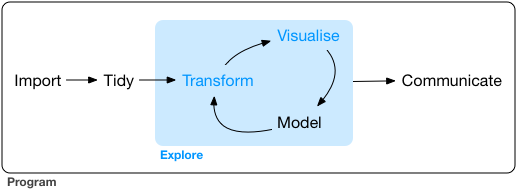
Wickham’s iterative approach to data science
The goal for this project is to develop a predictive model that will forecast the probability of WNV presence in 138 mosquito traps around Chicago over the course of a season. WNV is a communicable disease that is spread through its most common vector, mosquitoes. Most people infected with WNV develop no symptoms, but 1% will develop neurological symptoms including headache, high fever, neck stiffness, disorientation, coma, tremors, seizures, or paralysis2. There are no medical treatments or cures for WNV, so preventative measures are required to reduce infection to the human population. Local community methods of mosquito control include reduction of larval habitats and applying insecticides targeting larvae or adult mosquitoes.
Being able to predict the most likely sites of WNV outbreak is highly valuable to reduce the financial and human cost of over-application of insecticides. This project will focus on developing a deeper understanding of the problem using visuals and then develop a few relatively simple predictive models based on geographic information, weather conditions, presence of mosquito species, and historical trends of mosquito populations to predict the presence of WNV in the Chicago area.
Data briefing
Kaggle supplies five data sets for the competition, three of which can be used in model training. The train.csv file includes several variables associated with each West Nile Virus test including the trap id, geo-coordinates, date, species of mosquito present, number of mosquitoes present, and a binary variable indicating the presence or absence of West Nile Virus (WnvPresent), our target variable. The test.csv contains all the same features as the train.csv file except the number of mosquitoes present and the target WnvPresent variable. These data sets were obtained from West Nile Virus testing period between 2007 and 2014 with the training set containing the odd years and the test set containing the even years. The weather.csv file contains historic weather data collected at the O’Hare and Midway airports concurrent with the mosquito testing period. The spray.csv file includes the date and location of chemical spraying conducted by the city during 2011 and 2013. Since this spray data set would only have a large impact during one of the training years, I did not include the spray data in any of my models. For the weather data, since the differences in variables between O’Hare and Midway were generally small, I chose to use only the O’Hare data for all traps, rather than compute the closest station for each trap.
A large hypothetical variable influencing viral infection is population size. A larger population means there are more mosquitoes who can become infected, but it also increases the number of interactions between hosts, allowing faster spread of virus from individual to individual. The size of the population can be estimated from the number of mosquitoes found in each trap. However, this variable is not present in the test set, and will need to be imputed from other variables before a final model can be fit to the presence of West Nile using population as an input.
library(plyr)
library(tidyverse)
## Warning: Installed Rcpp (0.12.12) different from Rcpp used to build dplyr (0.12.11).
## Please reinstall dplyr to avoid random crashes or undefined behavior.## Loading tidyverse: ggplot2
## Loading tidyverse: tibble
## Loading tidyverse: tidyr
## Loading tidyverse: readr
## Loading tidyverse: purrr
## Loading tidyverse: dplyr## Conflicts with tidy packages ----------------------------------------------## arrange(): dplyr, plyr
## compact(): purrr, plyr
## count(): dplyr, plyr
## failwith(): dplyr, plyr
## filter(): dplyr, stats
## id(): dplyr, plyr
## lag(): dplyr, stats
## mutate(): dplyr, plyr
## rename(): dplyr, plyr
## summarise(): dplyr, plyr
## summarize(): dplyr, plyrload("west-nile/train.RData")
load("west-nile/test.RData")
ggplot(train, aes(x=WnvPresent, y=NumMosquitos)) +
geom_jitter(aes(color=WnvPresent)) +
ggtitle("Number of mosquitoes in West Nile \nVirus negative and positive traps") +
xlab("West Nile Virus present in trap") + ylab("Number of mosquitoes in trap")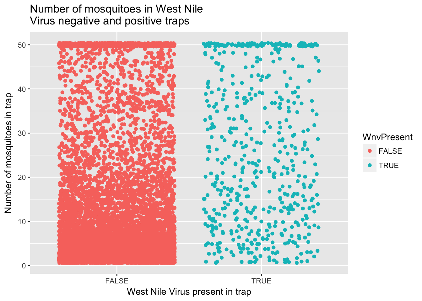
Based on this initial data exploration, I will first try and develop a model that predicts the number of mosquitoes in each trap and then use that predicted value as a variable in a model for WNV presence. For predicting the number of mosquitoes, I will first attempt using weather variables and weekly historic averages. Before modeling, I examined scatterplots of various input variables against mosquito counts, like the graph below comparing temperature to mosquito counts.
ggplot(train, aes(x=Tavg, y=Mosq_count)) +
  geom_jitter() +
  geom_smooth(method = lm) +
  ggtitle("Number of mosquitoes vs average daily temperature") +
  xlab("Average daily temperature, degree F") + ylab("Number of mosquitoes per trap")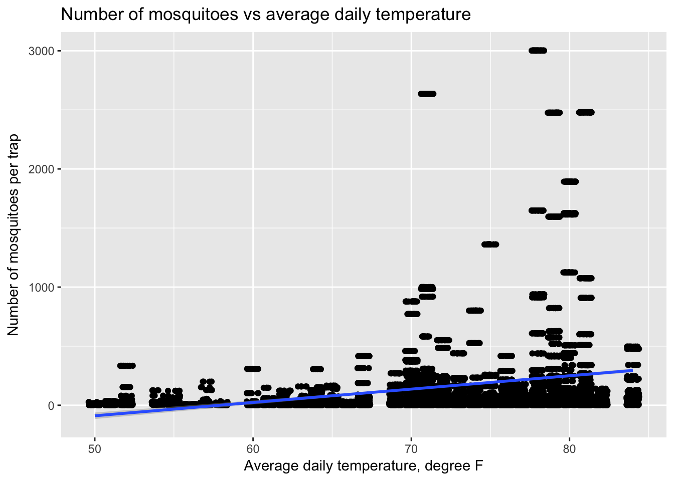
Tidying and transforming data
I cleaned up the weather and training data sets to impute missing values and delete non-informative columns. I next engineered several attributes from existing variables that I thought would be useful. Moving averages of temperature and precipitation, as well as weekly averages in overall mosquito counts were added to weather and training respectively. The code for variable engineering scripts (01_weather.R, 02_train_test.R) can be found in the src folder in the GitHub repo.
Modeling: Linear regression to predict mosquito population
For this first round of modeling, I will use linear regression to predict the number of mosquitoes using weather data and historical averages per week. I expect that higher average temperatures and greater moisture should have a positive effect on the mosquito population.
library(caret)## Loading required package: lattice##
## Attaching package: 'caret'## The following object is masked from 'package:purrr':
##
## liftset.seed(123)
split <- createDataPartition(y = train$NumMosquitos, p = 0.75, list = FALSE)
number_train <- train[split,]
number_valid <- train[-split,]
lm_variables <- c("Tmax",
"Tmin",
"Tavg",
"DewPoint",
"WetBulb",
"Sunrise",
"Sunset",
"PrecipTotal",
"ResultSpeed",
"ma3",
"ma5",
"ma10",
"precip3d",
"precip5d",
"precip10d")
lm_variables <- paste(lm_variables, collapse = "+")
fmla <- as.formula(paste("NumMosquitos", lm_variables, sep = "~"))
lm1 <- train(form = fmla,
data = number_train,
method = "lm")
number_train$lmNumMosq <- predict(lm1, newdata = number_train)
number_valid$lmNumMosq <- predict(lm1, newdata = number_valid)
train$lmNumMosq <- predict(lm1, newdata = train)
test$lmNumMosq <- predict(lm1, newdata = test)
summary(lm1)##
## Call:
## lm(formula = .outcome ~ ., data = dat)
##
## Residuals:
## Min 1Q Median 3Q Max
## -43.994 -10.576 -5.249 4.424 48.984
##
## Coefficients:
## Estimate Std. Error t value Pr(>|t|)
## (Intercept) -211.35042 28.81977 -7.334 2.46e-13 ***
## Tmax 1.52788 0.39822 3.837 0.000126 ***
## Tmin 1.96311 0.39673 4.948 7.65e-07 ***
## Tavg -3.66666 0.78568 -4.667 3.11e-06 ***
## DewPoint -0.81267 0.13950 -5.826 5.92e-09 ***
## WetBulb 1.10331 0.21191 5.207 1.97e-07 ***
## Sunrise 0.09426 0.01627 5.792 7.22e-09 ***
## Sunset 0.06936 0.01210 5.733 1.02e-08 ***
## PrecipTotal -0.46272 0.45810 -1.010 0.312492
## ResultSpeed 0.28297 0.06584 4.298 1.74e-05 ***
## ma3 0.59189 0.12213 4.846 1.28e-06 ***
## ma5 -0.70982 0.13854 -5.124 3.07e-07 ***
## ma10 0.71418 0.09174 7.785 7.89e-15 ***
## precip3d -36.36560 1.61641 -22.498 < 2e-16 ***
## precip5d 45.13598 2.27255 19.861 < 2e-16 ***
## precip10d 4.07897 1.53368 2.660 0.007839 **
## ---
## Signif. codes: 0 '***' 0.001 '**' 0.01 '*' 0.05 '.' 0.1 ' ' 1
##
## Residual standard error: 15.17 on 7866 degrees of freedom
## Multiple R-squared: 0.1198, Adjusted R-squared: 0.1181
## F-statistic: 71.37 on 15 and 7866 DF, p-value: < 2.2e-16Evaluate linear model for predicting mosquito number
The R^2 of the first model is 0.11, meaning that only 11% of observed mosquito population variation is explained by our weather model. To further evaluate the linear regression model, we can examine the residual errors against predicted numbers in the training data.
print(paste("RMSE score of lm1 on training data: ", round(RMSE(number_train$lmNumMosq, number_train$NumMosquitos), 1)))## [1] "RMSE score of lm1 on training data: 15.2"print(paste("RMSE score of lm1 on validation data: ", round(RMSE(number_valid$lmNumMosq, number_valid$NumMosquitos), 1)))## [1] "RMSE score of lm1 on validation data: 15.3"ggplot(data = number_valid, aes(x=lmNumMosq, y=(NumMosquitos - lmNumMosq))) +
geom_point(alpha = 0.05) +
ggtitle("Residual plot for estimating Mosquito number using linear model on weather data") +
xlab("Predicted number of mosquitoes in training set") +
ylab("Residual error (Actual - Predicted)") +
stat_smooth(method=lm)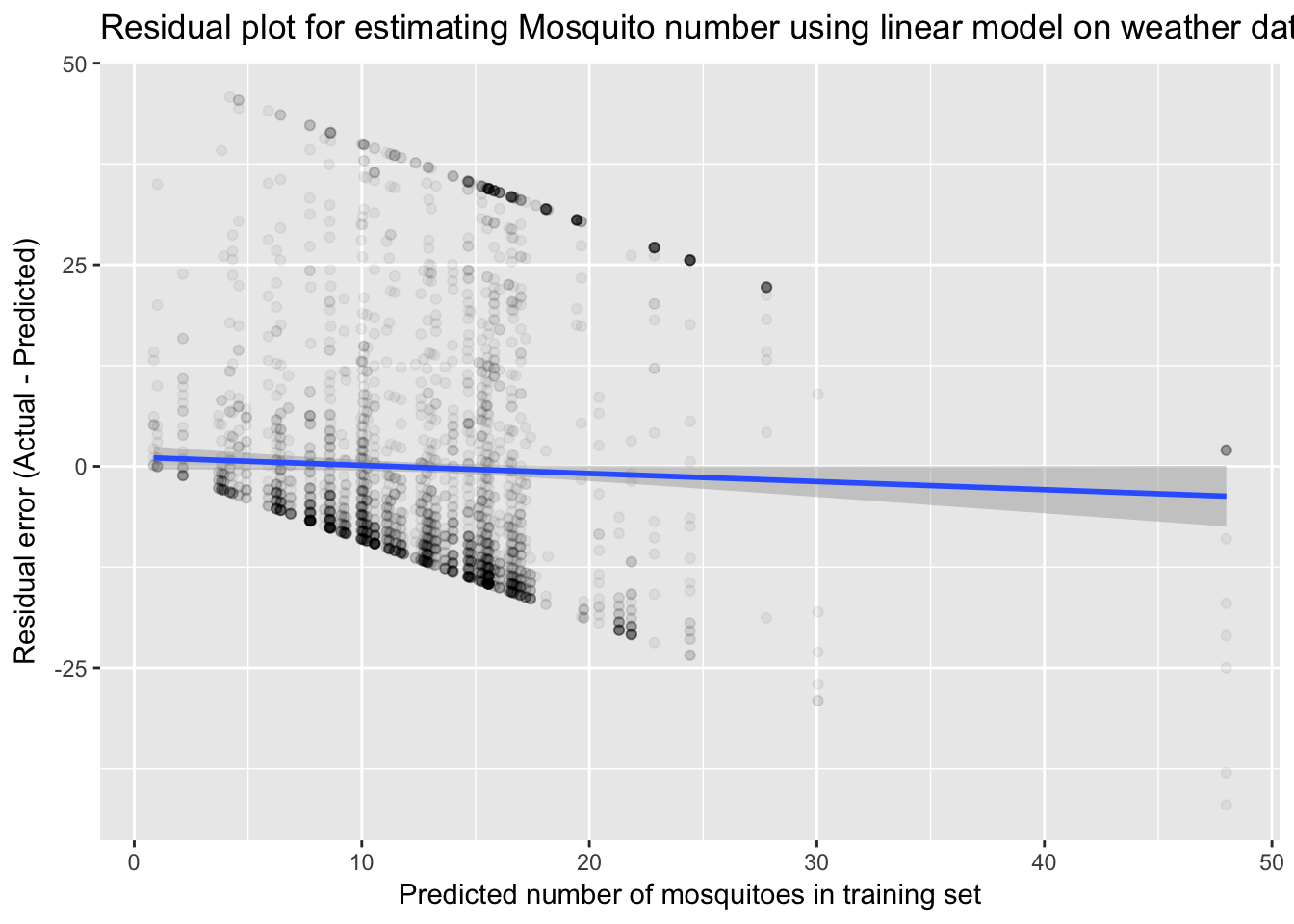
The residual plot appears to show bias in overestimating mosquitoes at the low end and underestimating at the high end. However, the trend shows that this is indeed zero. The odd shape is due to the fact that our actual values are bounded from 1-50. Let’s now include historical averages for each week in the year. We can also remove some variables that were not significantly informative in the previous model.
lm_variables2 <- c("WeekAvgMos",
                  "Tavg",
                  "Tmin",
                  "WetBulb",
                  "ResultSpeed",
                  "ma5",
                  "ma10",
                  "precip5d")

lm_variables2 <- paste(lm_variables2, collapse = "+")
fmla2 <- as.formula(paste("NumMosquitos", lm_variables2, sep = "~"))

lm2 <- train(form = fmla2,
             data = number_train,
             method = "lm")

number_train$lm2NumMosq <- predict(lm2, newdata = number_train)

number_valid$lm2NumMosq <- predict(lm2, newdata = number_valid)

train$lm2NumMosq <- predict(lm2, newdata = train)

test$lm2NumMosq <- predict(lm2, newdata = test)

summary(lm2)
##
## Call:
## lm(formula = .outcome ~ ., data = dat)
##
## Residuals:
## Min 1Q Median 3Q Max
## -17.387 -11.454 -5.746 4.716 47.520
##
## Coefficients:
## Estimate Std. Error t value Pr(>|t|)
## (Intercept) -14.27825 3.09657 -4.611 4.07e-06 ***
## WeekAvgMos 0.83001 0.06830 12.153 < 2e-16 ***
## Tavg 0.20815 0.08394 2.480 0.0132 *
## Tmin 0.06859 0.07050 0.973 0.3306
## WetBulb -0.05817 0.08327 -0.699 0.4848
## ResultSpeed 0.08779 0.06540 1.342 0.1795
## ma5 0.02772 0.08301 0.334 0.7384
## ma10 -0.02540 0.09034 -0.281 0.7786
## precip5d 0.87161 0.67629 1.289 0.1975
## ---
## Signif. codes: 0 '***' 0.001 '**' 0.01 '*' 0.05 '.' 0.1 ' ' 1
##
## Residual standard error: 15.63 on 7873 degrees of freedom
## Multiple R-squared: 0.06467, Adjusted R-squared: 0.06372
## F-statistic: 68.04 on 8 and 7873 DF, p-value: < 2.2e-16print(paste("RMSE score of lm2 on training data: ", round(RMSE(number_train$lm2NumMosq, number_train$NumMosquitos), 1)))## [1] "RMSE score of lm2 on training data: 15.6"print(paste("RMSE score of lm2 on validation data: ", round(RMSE(number_valid$lm2NumMosq, number_valid$NumMosquitos), 1)))## [1] "RMSE score of lm2 on validation data: 15.6"This results in an even lower R^2 value of 0.06 and a higher RMSE error score. Since these values are against the training data this could mean that the first model is overfitting the training set. This is entirely possible since it included a larger number of input variables. The best way to test this is testing and evaluating against our hold-out data. The hold-out RMSE for lm1 was 783.6 and for lm2 was 799.1, so here again we are better with the first model.
A further look at mosquito number distribution
To get a better estimate of mosquito counts, I next wanted to go back and examine the distribution of the Mosquito counts a bit further. The total number with each observation is capped between 1 and 50 mosquitoes. Since there are several rows of data for each trap/date combination when one trap has the full 50 mosquitos, this is likely how the mosquitos are split up for testing. Mosquitoes are collected in the traps and split up into groups with no more than 50 mosquitos, recorded for Species and then tested for WNV. To help correct for this, I added up all of the multiple observations per trap to This distribution is not at all near normal or gaussian, as you can see by the histograms below, and instead resembles a Poisson distribution with no zeros and a cap at 50. Compare the QQplots of Normal and Poisson (\(\lambda = 12.8\)) distributions against log2 transformed number of mosquitos.
Mosq_number <- train %>% group_by(Trap, Date) %>% summarise(Mosq_count = sum(NumMosquitos), nrows = n())

poissonlist <- rpois(1000, 12.8)
poissonlist[poissonlist == 0] <- 1

par(mfcol = c(2,2))
hist(Mosq_number$Mosq_count, col = "lightblue", main = "Histogram mosquito number")
qqnorm(log2(Mosq_number$Mosq_count), main = "QQPlot Normal distribution")
hist(log2(Mosq_number$Mosq_count), col = "lightblue", main = "Histogram log2 mosquito number")
qqplot(poissonlist, log2(train$Mosq_count), main = "QQPlot Poisson with 0 removed")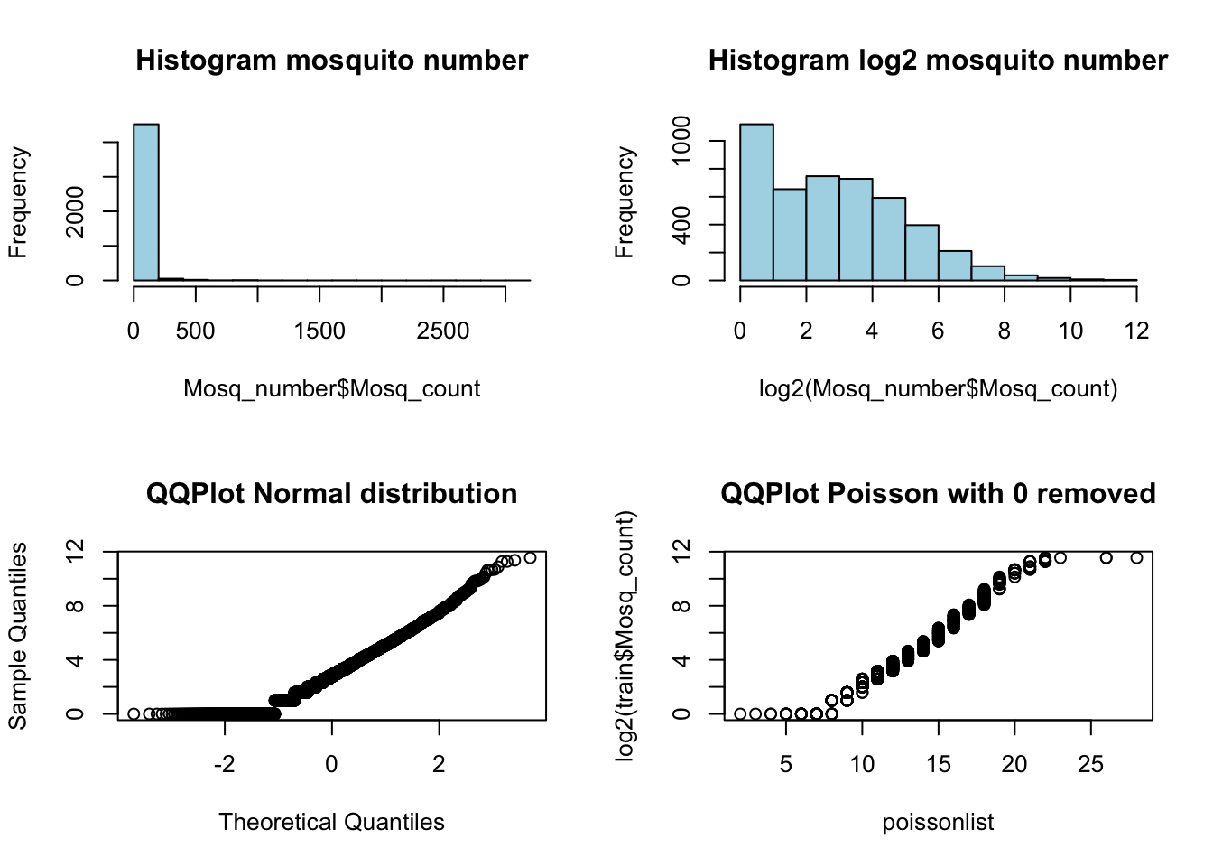
par(mfcol = c(1,1))Modeling: Poisson Regression
poisson <- train(form = fmla,
             data = number_train,
             method = "glm",
             family = "poisson")

number_train$poissonNumMosq <- predict(poisson, newdata = number_train)
number_valid$poissonNumMosq <- predict(poisson, newdata = number_valid)

train$poissonNumMosq <- predict(poisson, newdata = train)

test$poissonNumMosq <- predict(poisson, newdata = test)

summary(poisson)
##
## Call:
## NULL
##
## Deviance Residuals:
## Min 1Q Median 3Q Max
## -9.323 -3.574 -1.959 1.322 12.737
##
## Coefficients:
## Estimate Std. Error z value Pr(>|z|)
## (Intercept) -1.662e+01 5.705e-01 -29.137 < 2e-16 ***
## Tmax 1.039e-01 7.372e-03 14.088 < 2e-16 ***
## Tmin 1.418e-01 7.404e-03 19.152 < 2e-16 ***
## Tavg -2.513e-01 1.450e-02 -17.324 < 2e-16 ***
## DewPoint -6.724e-02 2.798e-03 -24.034 < 2e-16 ***
## WetBulb 8.645e-02 4.299e-03 20.110 < 2e-16 ***
## Sunrise 8.011e-03 3.140e-04 25.511 < 2e-16 ***
## Sunset 5.778e-03 2.411e-04 23.965 < 2e-16 ***
## PrecipTotal -1.146e-01 1.154e-02 -9.932 < 2e-16 ***
## ResultSpeed 3.080e-02 1.214e-03 25.365 < 2e-16 ***
## ma3 4.648e-02 2.304e-03 20.172 < 2e-16 ***
## ma5 -6.352e-02 2.612e-03 -24.320 < 2e-16 ***
## ma10 6.718e-02 1.763e-03 38.097 < 2e-16 ***
## precip3d -1.848e+00 2.142e-02 -86.233 < 2e-16 ***
## precip5d 2.198e+00 3.065e-02 71.714 < 2e-16 ***
## precip10d 1.973e-01 2.546e-02 7.750 9.21e-15 ***
## ---
## Signif. codes: 0 '***' 0.001 '**' 0.01 '*' 0.05 '.' 0.1 ' ' 1
##
## (Dispersion parameter for poisson family taken to be 1)
##
## Null deviance: 134193 on 7881 degrees of freedom
## Residual deviance: 116462 on 7866 degrees of freedom
## AIC: 145001
##
## Number of Fisher Scoring iterations: 5print(paste("RMSE score of Poisson regression on validation set: ", round(RMSE(number_valid$poissonNumMosq, number_valid$NumMosquitos), 1)))## [1] "RMSE score of Poisson regression on validation set: 15.2"This is slightly better than standard linear regression, with an RMSE of 778.5. I will this estimate for the number of mosquitos in the final prediction for WNV in the test set.
Examining the effect of geography and location
In addition to mosquito population size and weather variables, there is likely to be an effect based on a trap’s geographic location. Next, I wanted to visually examine the relationship between geography and West Nile presence. In other words, I wanted to make some cool maps! First I created a map of Wnv incidents as a density plot. Here, the density is derived from the overall positive count for each trap.
library(ggmap)
chicago <- get_map("Chicago")
## Map from URL : http://maps.googleapis.com/maps/api/staticmap?center=Chicago&zoom=10&size=640x640&scale=2&maptype=terrain&language=en-EN&sensor=false## Information from URL : http://maps.googleapis.com/maps/api/geocode/json?address=Chicago&sensor=falsewnpositive <- filter(train, WnvPresent == TRUE)
load("west-nile/traps.RData")
ggmap(chicago) + geom_density2d(data = wnpositive, aes(x = Longitude, y = Latitude), size = 0.3) +
stat_density2d(data = wnpositive, aes(x = Longitude, y = Latitude, fill = ..level.., alpha = ..level..), size = 0.01, bins = 16, geom = "polygon") +
scale_fill_gradient(name="Number of WNV+", low = "green", high = "red") +
scale_alpha(range = c(0, 0.3), guide = FALSE) +
ggtitle("Heat map of West Nile Virus positive traps") +
xlab("Longitude") + ylab("Latitude") +
geom_point(data = traps, aes(x = Longitude, y = Latitude), shape = 4)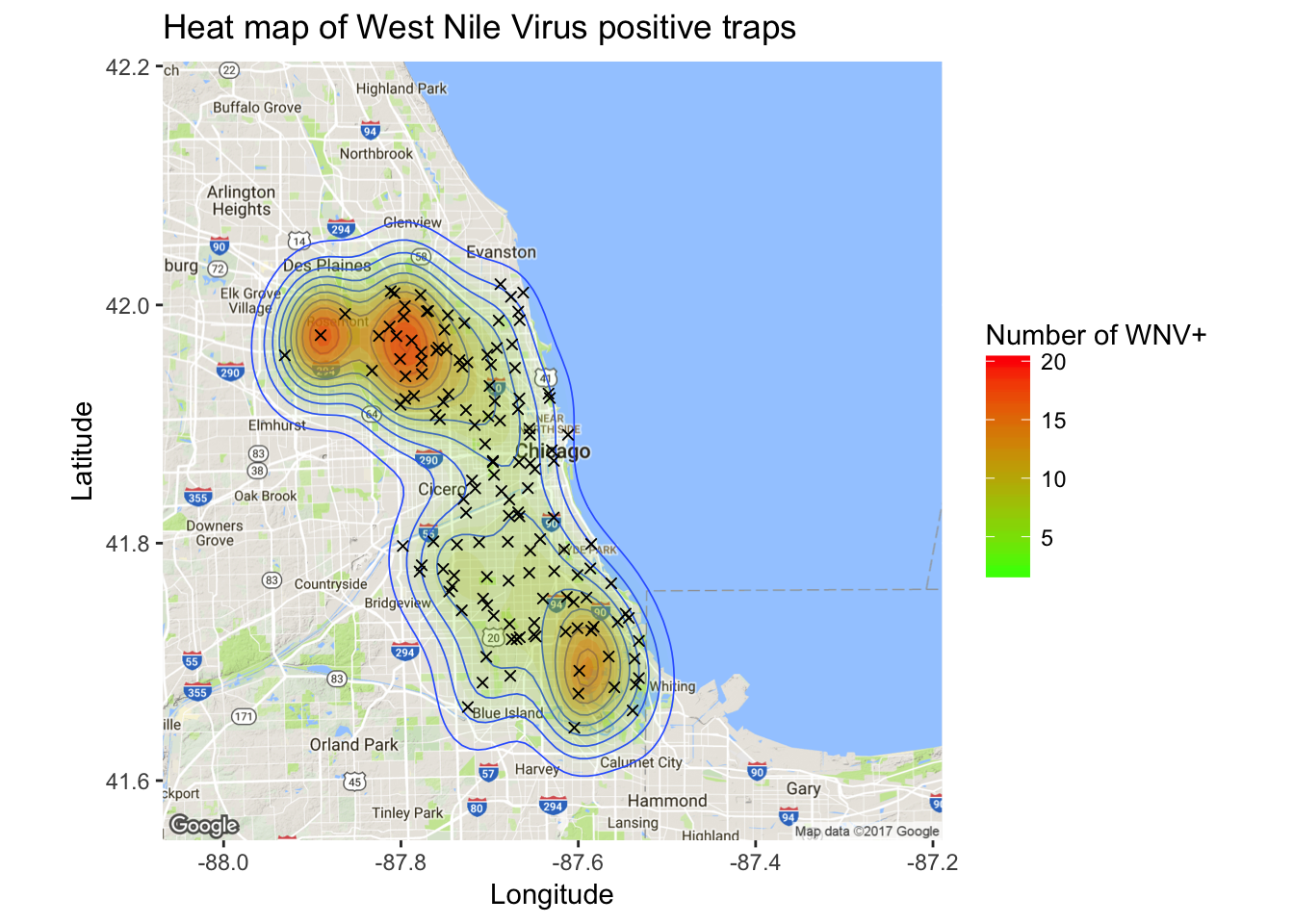
It’s clear from the density map that there are hotspot traps where West Nile is more common than others, and this appears to influence nearby traps.
Now that we have a good 2-dimensional view of the occurence of WNV, I next wanted to get a sense of how this pattern of West Nile Virus changed over time in relation to the geography. I did this by creating an animated version of this map using a new R package called gganimate. I chose to remove the background map of Chicago to get a clearer visual of positive vs negative cases. This animation uses the new gganimate package.
library(gganimate)
library(animation)

byyearweek <- group_by(train, Year, Week) %>% summarize(weekly_avg_mosq = mean(NumMosquitos))
train$timepoint <- ((train$Year - 2007) + (train$Week / 52)) * 52

map_mosq <- ggplot(train, aes(x=Longitude, y=Latitude,
                                  size=NumMosquitos,
                                  color=WnvPresent,
                                  frame=timepoint)) + geom_point(alpha = .5) +
                                  ggtitle("Animated map of mosquitos and \npresence of West Nile Virus in Chicago \n")

animated_map_mosq <- gganimate(map_mosq, interval=0.5)
animated_map_mosq
Mosquito map
There are various ways to incorporate geography into a predictive model. I could incorporate the trap id in the model or I could incorporate the longitude and latitude for very high precision. The longitude/latitude method would require a decision tree or other model that allows for breaking up or clustering the locations in some non-linear way.
Instead, I am choosing to group the traps into clusters and include the cluster as a modeling parameter. The reasoning for this is that suspect that the true risk based on geography has a much lower actual precision than our ability to define latitude or longitude.
Data preparation: Clustering traps according to location and WNV presence
To create clusters of traps I want to incorporate not only geographical information, but WNV rate as well. This will help to create breaks in my clusters that are informative for predicting future WNV rate. The code for clustering is found in the “04_geo_cluster.R” script.
load("west-nile/train_geo.RData")
load("west-nile/test_geo.RData")
load("west-nile/trap_geo_hot.RData")

ggplot(trap_geo_hot, aes(Longitude, Latitude, color = geo.hot.cl)) + geom_point()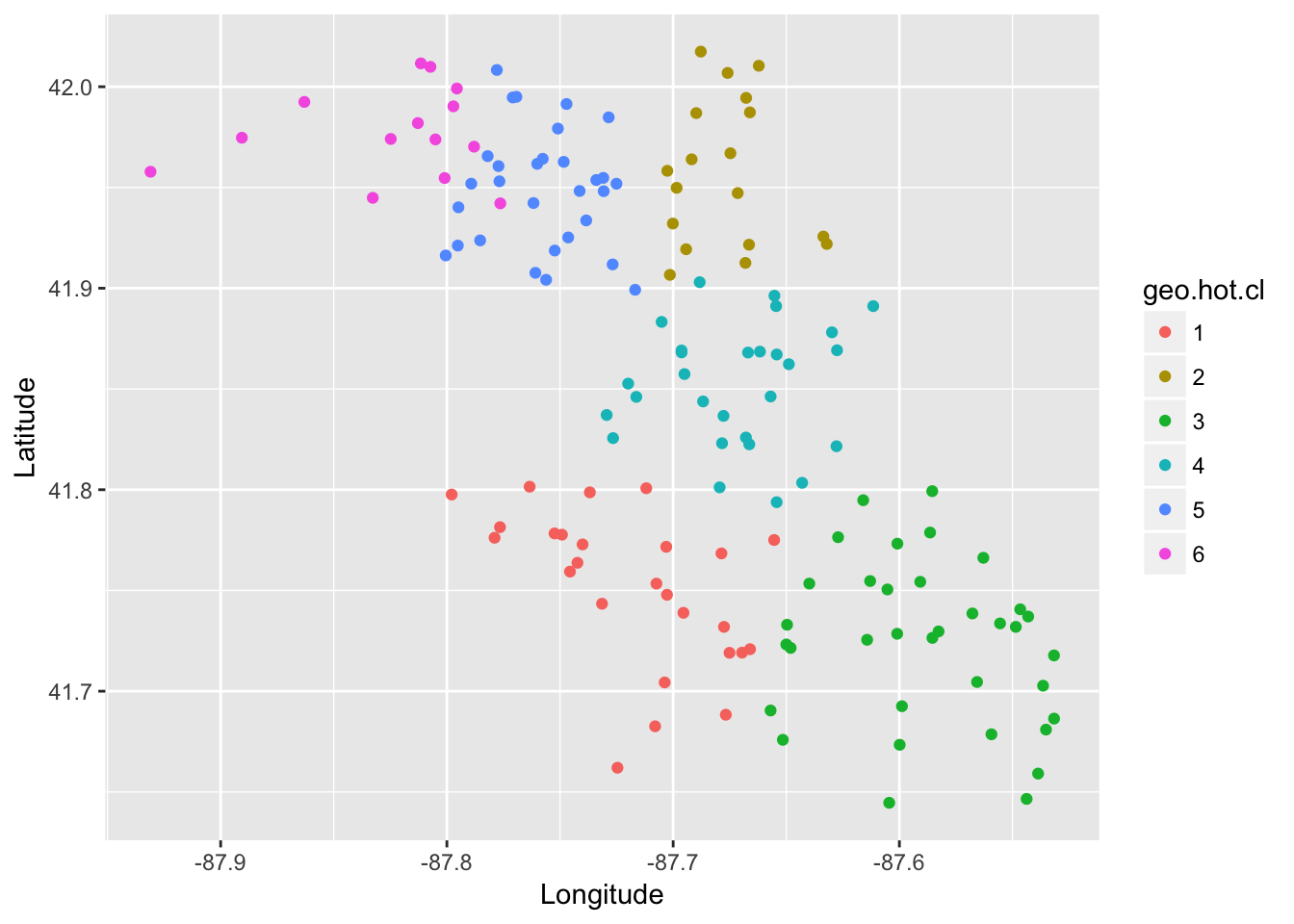
ggmap(chicago) + geom_density2d(data = wnpositive, aes(x = Longitude, y = Latitude), size = 0.3) +
  stat_density2d(data = wnpositive, aes(x = Longitude, y = Latitude, fill = ..level.., alpha = ..level..), size = 0.01,
    bins = 16, geom = "polygon") +
  scale_fill_gradient(name="Number of WNV+", low = "green", high = "red") +
  scale_alpha(range = c(0, 0.3), guide = FALSE) +
  ggtitle("Heat map of West Nile Virus positive traps") +
  xlab("Longitude") + ylab("Latitude") +
  geom_point(data = trap_geo_hot, aes(x = Longitude, y = Latitude, shape = geo.hot.cl)) + scale_shape_discrete(name = "Trap Cluster")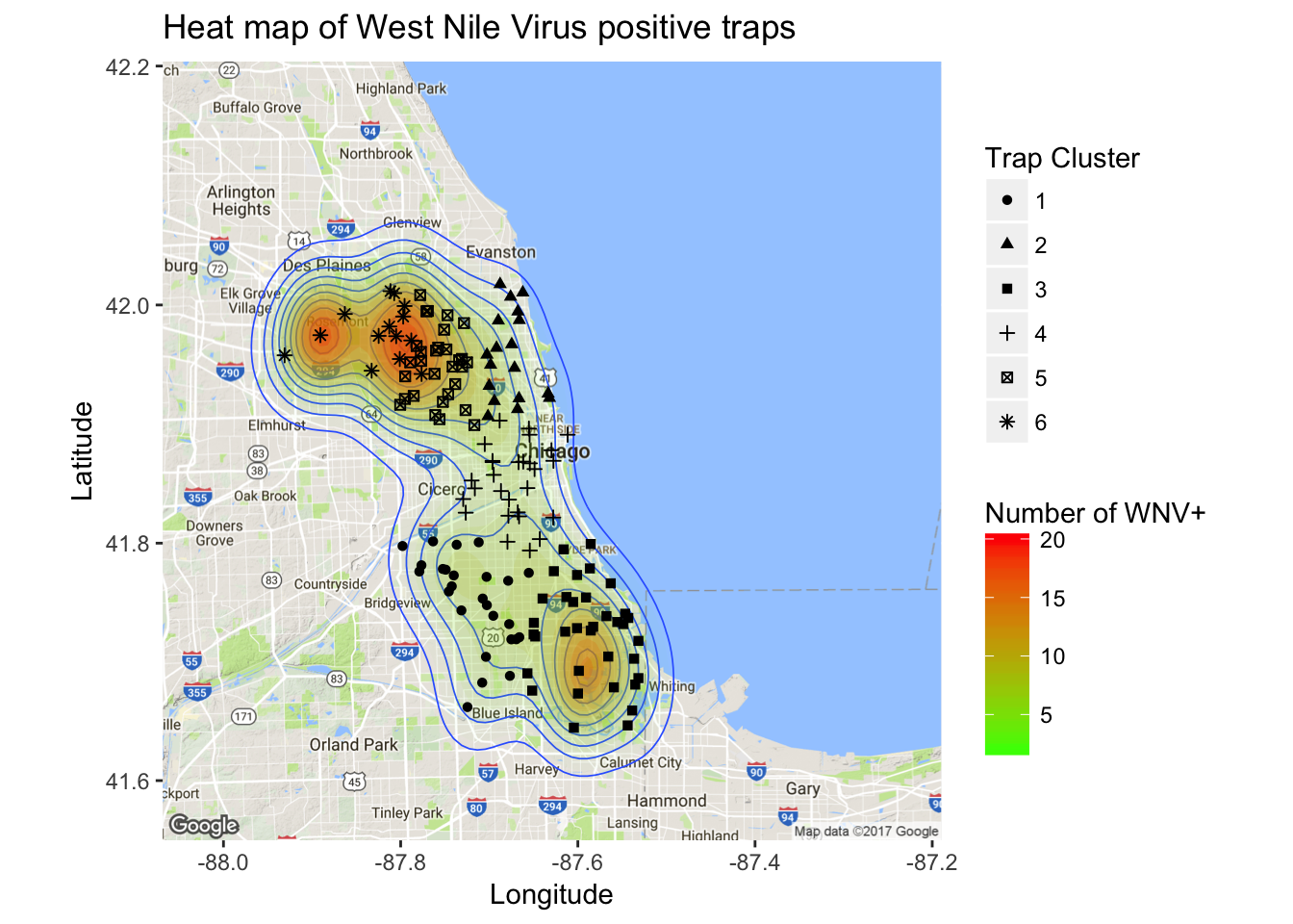
Now that I have some geographical clusters for each trap and a good handle on predicting mosquito number, I can use those as input variables for the ultimate target, WNV probability. I will be comparing several different models for my next post.
Bibliography
Wickham, H., R for Data Science.↩